Generalization Gaps of VAE

1. Generalization of Probabilistic Models

The goal of probabilistic modelling is to learn a model $p_\theta(x)$ to fit the training dataset $\mathcal{X}_{train}=\{x_1,\cdots,x_N\}\sim p_d(x)$, where $p_d(x)$ is the unknown data distribution. A common training criterion is the maximum likelihood learning:

The generalization of the $p_\theta(x)$ can be evaluated using the test log-likelihood $\frac{1}{M}\sum_{m=1}^M \log p_\theta(x'_m)$ with the test dataset $\mathcal{X}_{test}=\{x'_1,…,x'_M\}\sim p_d(x)$. This definition of generalization has an important practical implicaition: by using the mdoel $p_\theta(x)$, we can design a compression algorithm to compress a data $x'$ losslessly into a binary string whose length is approximately $-\log_2 p_\theta(x')$. Therefore, a better generalization, as measured by the test log-likelihood, translates to enhanced performance in practical lossless compression. A detailed discussion on the this connection can be found in David MacKay's textbook.

Furthermore, it's noteworthy that this perspective on lossless compression has been instrumental in recent efforts to understand the generalization properties of large language models, see the video by Ilya Sutskever for a discussion.

2. Introduction of VAE

Variational Auto-Encoder (VAE) is a latent variable model with the form

where the $p_\theta(x|z)$ is the deocder and $p(z)$ is the prior. When $p_\theta(x|z)$ is parameterized by a neural network, the integration over $z$ is is usually not tractable. A lower-bound of the log-likelihood can be used, which is refered to as the ELBO

where $p_\theta(z|x_n)$ is the true posterior $p_\theta(z|x_n)\propto p_\theta(x_n|z)p(z)$. The VAE has been successfully used in lossless compression and the test compression length is approximately equal to the negative ($\text{log}_2$) ELBO, see the BB-ANS paper for a practical guidence. Therefore, we will then focus on the generalization of the ELBO.

1. Generalization Gaps of VAE

This empirical ELBO objective can be further represented as a combination of a model empirical approximation and an amortized inference empirical approximation:

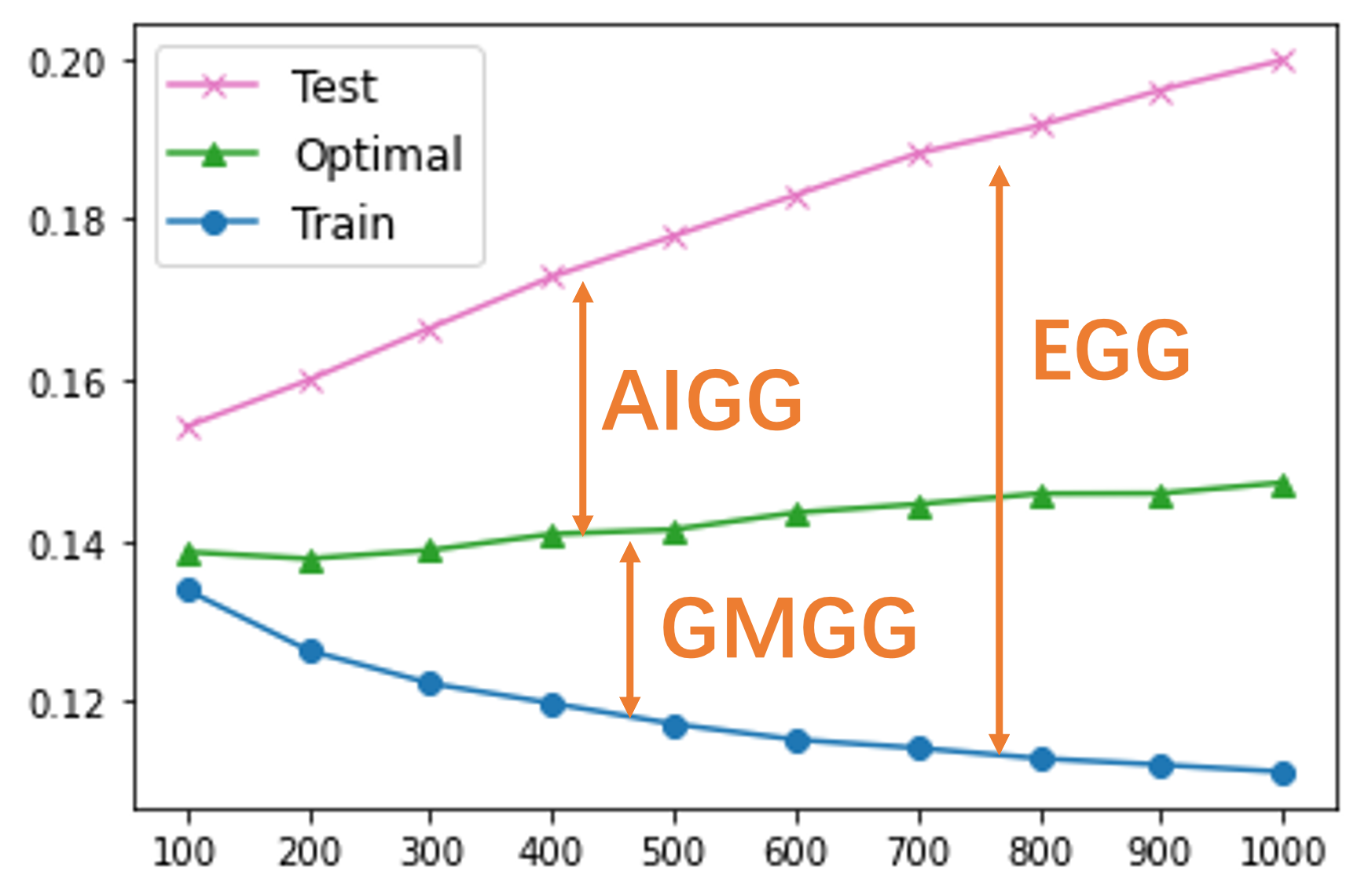
If either the decoder $p_\theta(x|z)$ or the encoder $q_\phi(z|x)$ is overly flexible, it can cause the VAE to overfit to the training data. We can define the ELBO generalization gap (EGG) as the difference between the training and test ELBO

where $\theta^*_N,\phi^*_N$ are defined as the optimal parameters for training the empirical ELBO

We notice that $\phi^*_N$ is also the optimal parameter of the empirical amortized inference

For simplicity, considering a flexible amortized inference network, we can assume that for any training data point $x_n\in\mathcal{X}_{train}$, the $q_{\phi^*_N}(z|x_m')$ can generate the optimal posterior within the variational family $\mathcal{Q}$:

However, when $q_{\phi^*}(z|x_n)$ overfits to $\mathcal{X}_{train}$, $q_{\phi^*}(z|x'_m)$ may not be a good approximation to the true posterior $p_{\theta^*_N}(z|x_m')$ for test data $x'_m\in \mathcal{X}_{test}$. This discrepancy can lead to a suboptimal test ELBO.

To illustrate the generalization of the amortized inference, we denote the $\phi^*_M$ as the optimal realizable parameter of the amortized inference for the test data $x'_m\in \mathcal{X}_{test}$:

Similarly, we assume that $q_{\phi^*_M}(z|x_m')$ can generate the optimal posterior within the variational family $\mathcal{Q}$ for a flexible $q_\phi(z|x)$,

We then define the amortized inference generalization gap (AIGG) as the difference between two averaged KL divergences

Intuitively, AIGG assesses the proximity of the posterior $q_{\phi^*_N}(z|x'_m)$, — which is derived from the amortized network trained on $\mathcal{X}_{train}$ — to the optimal realizable posterior for $x'_m\in\mathcal{X}_{test}$. Equivalently, the AIGG can also be written as the difference between two ELBOs with $\phi^*_M$ and $\phi^*_N$ respectively:

It is important to emphasize that this gap cannot be reduced by simply using a more flexible variational family $\mathcal{Q}$. While this might reduce the $\mathrm{KL} (q_{\phi^*_N}(z|x_n)||p_{\theta^*_N}(z|x_n))$ for the training data $x_n\in \mathcal{X}_{train}$, it would not explicitly encourage a smaller AIGG.

The AIGG is caused by the overfitting of the amortized inference (encoder). To understand the generalization property of the decoder, we can further rewrite the EGG by subtracting and adding the term $\frac{1}{M}\sum_{m=1}^M \mathrm{ELBO}(x'_m,\theta^*_N,\phi^*_M)$:

where the second term is just the AIGG. Meanwhile, we define the expression in the first term, which is the difference between the training and test ELBO using the optimal amortized inference parameters $\phi^*_N,\phi^*_M$ respectively, as the Generative Model Generalization Gap (GMGG), which can isolate the degree of which part affect the overall generalization.

With this in perspective, we can express the EGG as a combination of both gaps:

This decomposition highlights that the VAE's generalization performance is influenced by the generalization capabilities of both the generative model and the amortized inference.

3. Visualization of the Generalizatio Gaps

To visualize the generalization gaps, we trained a VAE on the Binary MNIST training dataset for 1,000 epochs. For every 100 epochs, we fix the decoder $p_\theta(x|z)$ and only train $q_\phi(z|x)$ for 1k epochs on the test data to obtain the estimation of the optimal amortized posterior $q_{\phi_M^*}$.

We can see the VAE overfits the training dataset easily. We also notice that utilizing the test ELBO with the test-time optimal inference strategy, the test BPD (green) appears largely stable, showing just a minor increase during training. This pattern hints at the overfitting of the generative model (decoder) being less pronounced compared to that of the amortized inference network (encoder). Consequently, the primary source of significant overfitting is dominated by the overfitting of the amortized inference network.

Using this observation, we can design algorithm to alleviate the overfitting of the amortized inference. Please see our NeurIPS paper Generalization Gaps in Amortized Inference for the furthur discussion how to reduce the generalization gaps of VAE.