A Failure Case of VAE

The Variational Auto-Encoder (VAE) has been widely used to model complex data distributions. In this post, we discuss a simple but important failure mode of VAEs as well as a solution proposed in the paper Spread Divergences to fix the broken VAE. The code to reproduce the experiments behind the figures can be found here.

1. Introduction of VAE

Given a dataset $\{x_1,…,x_N\}$ sampled from some unknown data distribution $p_d(x)$, we are interested in using a model $p_\theta(x)$ to approximate $p_d(x)$. A classic way to learn $\theta$ is to minimize the KL divergence:

From the definition of "divergence", we know that:

The integration over $p_d(x)$ can be approximated by the Monte-Carlo method:

When $N \rightarrow \infty$, minimizing the KL divergence is equivalent to Maximum Likelihood Estimation (MLE). For a latent variable model $p_\theta(x)=\int p_\theta(x|z)p(z)dz$ with $p_\theta(x|z)$ parameterized by a neural network, the log-likelihood $\log p_\theta(x)$ is usually intractable. We can instead maximize the Evidence Lower Bound (ELBO):

Where $q_\phi(z|x)$ is the amortized posterior that is introduced to approximate the true model posterior $p_\theta(z|x) \propto p(x|z)p(z)$. The training objective becomes maximizing $\frac{1}{N}\sum_{n=1}^N \mathrm{ELBO}(x_n,\theta,\phi)$.

2. A failure case

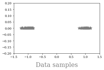
Let’s consider the following data generation process for data $x\sim p_d(x)$:

We also plot the data samples:

We attempt to learn this distribution with a VAE of the following form:

• $p_\theta(x|z)$: 2D Gaussian with learned mean and variance;
• $p(z)$: 1D Bernoulli with mean equal to 0.5;
• $q_\phi(z|x)$: 1D Bernoulli with learned mean.

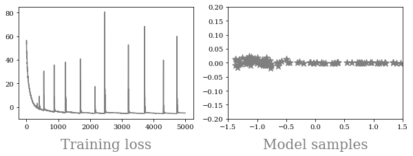
If we plot the training loss and samples from the resulting trained VAE we find that the training is unstable and the quality of the samples is bad.

2. Why the failure happens?

Computational: The y-axis of the $p_d(x)$ has 0 variance, and so the variance of the y-axis in $p_\theta(x|z)$ converges to 0 during training and the log likelihood becomes infinity.

Theoretical: The data distribution is a 1D manifold distribution that lies in a 2D space. Its density function is not well-defined (the distribution is not absolutely continuous w.r.t. Lebesgue measure.), so the KL divergence and MLE are ill-defined or cannot provide valid gradients for training. This problem has also been previously discussed in Wasserstein GAN.

3. A simple fix: spread KL divergence

A simple trick to fix the problem is adding the same amount of convolutional noise to both data distribution $p_d(x)$ and model $p_\theta(x)$. For example, we can choose a Gaussian noise distribution $n(\tilde{x}|x)=\mathrm{N}(x,\sigma_{fix}^2 I)$ and let:

We further define the spread KL divergence $\widetilde{\mathrm{KL}}_n(p_d(x)||p_\theta(x))$ as:

Our paper shows that for some certain noise distributions (e.g. Gaussian), we have:

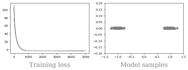
This provides a good estimation for $\mathrm{KL}(p_d(x)||p_\theta(x))$ and can provide valid gradients for training. When we train with spread KL divergence, the result becomes much better:

3. Conclusion

Even a simple model like VAE can fail in a seemingly straightforward situation due to both computational and theoretical reasons. Recognizing these pitfalls can help us design better models. A simple but effective fix is to spread the KL divergence, which provides valid training signals and fixes the problem.